In this post we are going to backtest a simple trend trading strategy. This simple trend trading strategy entails calculating the difference between 42 period SMA and 252 period SMA and then going long/short if the difference is greater than or lower than a certain regime variable SD. USD was on a roller coaster after the recent US Presidential Elections. Did you read the post on how to trade the US Presidential Elections? Getting back to our simple trend trading strategy, we will be using GBPUSD 30 minute data. We will be using Python scripting language to do the backtest. You should have Anaconda and Spyder installed on your computer before you proceed. Numpy and Pandas are two important modules that you should master.
Algorithmic trading is the new game in the town. More and more people are now using algorithmic trading. Do you know this that college kids are now running algorithmic trading systems from their dorms. If you are not giving much importance to algorithmic trading, then this is the time to start learning algorithmic trading. Did you take a look at our course Algorithmic Trading System Design? In this course we teach you step by step in simple terms how you can design and develop your own algorithmic trading system. Python is a popular language that is being used by big banks and hedge funds in designing and developing algorithmic trading systems. You should learn Python. Below is the code that implements our simple trend trading strategy backtest in Python.First we read the data from csv.
#trend trading strategy
import numpy as np
import pandas as pd
import matplotlib.pyplot as plt
#read the data from the csv file
data1 = pd.read_csv('E:/MarketData/GBPUSD30.csv', header=None)
data1.columns=['Date', 'Time', 'Open', 'High', 'Low', 'Close', 'Volume']
data1.shape
#show data
data1.head()
#plot the closing price
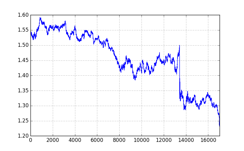
data1['Close'].plot(grid=True, figsize=(8, 5))
#add the 2 month and the 1 year moving average to the dataframe
data1['42SMA'] = np.round(pd.rolling_mean(data1['Close'], window=42), 2)
data1['252SMA'] = np.round(pd.rolling_mean(data1['Close'], window=252), 2)
data1[['Close', '42SMA', '252SMA']].tail()
This is the python code. First we read the GBPUSD M30 csv file. This is the output.
(17037, 7)
>>>
Date Time Open High Low Close Volume
0 2015.05.25 20:30 1.54680 1.54726 1.54659 1.54714 2174
1 2015.05.25 21:00 1.54715 1.54725 1.54695 1.54715 2140
2 2015.05.25 21:30 1.54716 1.54720 1.54704 1.54717 1526
3 2015.05.25 22:00 1.54718 1.54721 1.54679 1.54713 1646
4 2015.05.25 22:30 1.54712 1.54721 1.54692 1.54705 976
You can see we have a total of 17037 observations in our dataframe. We add 2 columns. One is the 42SMA and the other is 252SMA. This is what we get.
>> data1[‘Close’].plot(grid=True, figsize=(8, 5))
Close 42SMA 252SMA
17032 1.23872 1.25 1.28
17033 1.23153 1.25 1.28
17034 1.23396 1.25 1.28
17035 1.23777 1.25 1.28
17036 1.23557 1.25 1.28
Below is the plot of the closing price.
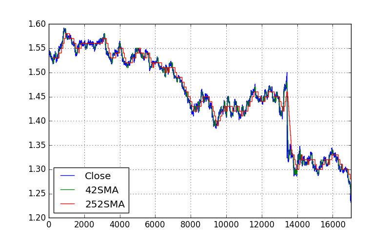
We need to calculate the difference between 42SMA and 252SMA and plot the new lines.
#plot the new lines
data1[['Close', '42SMA', '252SMA']].plot(grid=True, figsize=(8, 5))
#calculate the difference between 2 SMAs
data1['42SMA-252SMA'] = data1['42SMA'] - data1['252SMA']
data1['42SMA-252SMA'].tail()
This is the difference between the 2 SMAs.
17032 -0.03
17033 -0.03
17034 -0.03
17035 -0.03
17036 -0.03
Below is the plot of 42SMA and 252SMA.
Now we need to define the regime. A buy signal is generated when 42SMA is SD points above 252SMA. Similarly when 42SMA is SD points below 252SMA, a sell signal is generated. When 42SMA is +/- SD points within 252SMA no buy/sell signal is generated. In the code below we have chosen SD to be 0.01.
#define a regime
SD = 0.01
data1['Regime'] = np.where(data1['42SMA-252SMA'] > SD, 1, 0)
data1['Regime'] = np.where(data1['42SMA-252SMA'] < -SD, -1, data1['Regime'])
data1['Regime'].value_counts()
#plot the regime
data1['Regime'].plot(lw=1.5)
plt.ylim([-1.1, 1.1])
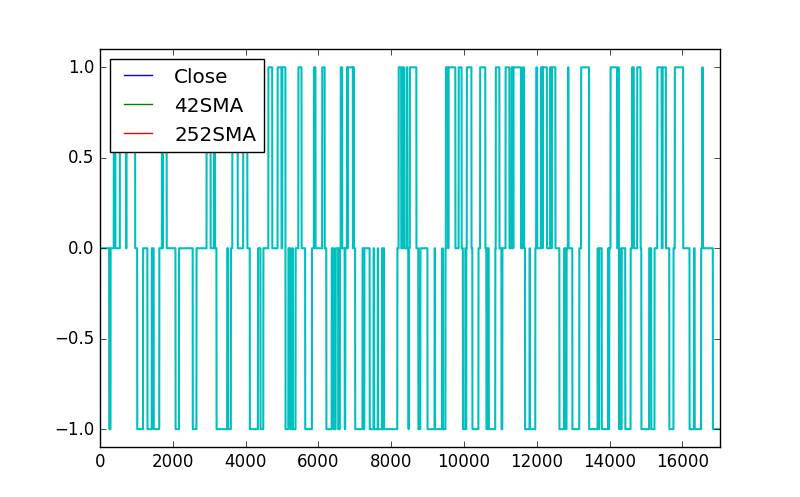
This is the regime data!
>> SD = 0.01
0 6404
-1 6213
1 4420
6404 observations have 42SMA within +/- SD points of 252SMA. 6213 observations have 42SMA SD point below 252SMA and 4420 observations have 42SMA SD point above 252SMA.Below is the python code for backtesting.
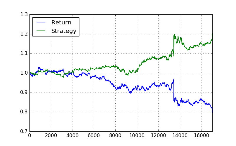
#backtesting the trend trading strategy
data1['Return'] = np.log(data1['Close'] / data1['Close'].shift(1))
data1['Strategy'] = data1['Regime'].shift(1) * data1['Return']
data1[['Return', 'Strategy']].cumsum().apply(np.exp).plot(grid=True, figsize=(8, 5))
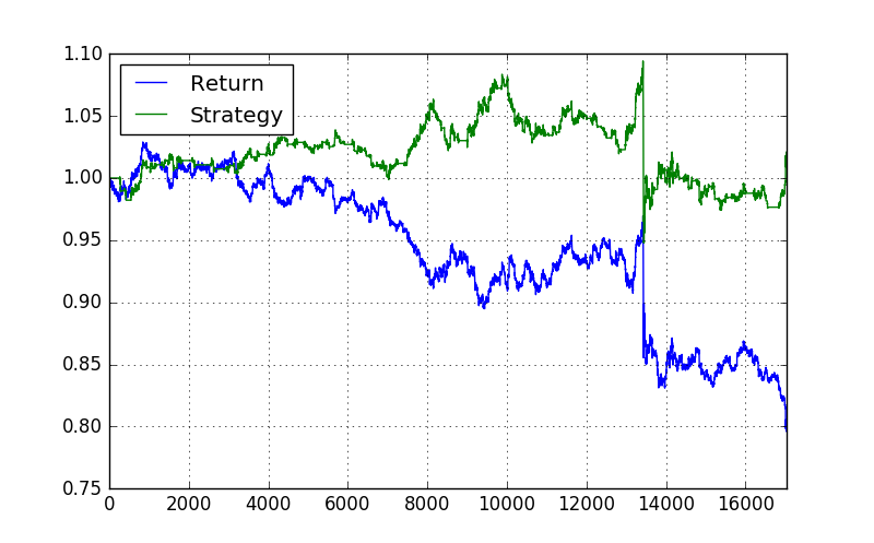
You can see in the above plot the strategy return which is positive and greater than the actual returns. It would be a good idea to change the SMA periods. You can change the SMA periods to 21 and 144. You can also change the regime variable SD to 0.02 or even 0.005. Use the above code and do the backtesting and see if you get better results. Did you take a look at Quantopian backtesting platform? Quantopian allows you to backtest your trading strategy using python code. Quantopian community is very large now. You can meet a lot of expert quants in the Quantopian community who can help you and answer your coding questions. You should frequently visit Quantopian as it has got a big active community.
R is another powerful scripting language that you can use in algorithmic trading. Did you read the post on how to develop autoregressive models using R? In this post I show you how to use the power of autoregression in predicting price. The problem in most financial models is that we use returns and try to build a model in it. When we calculate returns we are infact losing a lot of predictive power. We need to directly model price. This can give better predictions. In the future, I will write a few posts on how to do deep learning.in the above backtesting we didn’t take into account the spread when we enter and exit the market. But you can see the equity curve of this simple trend trading strategy is positive. We can improve upon this strategy and make it more robust. Algorithmic trading is all about building better predictive models. Did you read the post on how to use NNET Neural Network in predicting price?
You should focus on learning Python and R in the beginning. When you become an expert at Python and R, you should also try to learn C++ and Java. Both C++ and Java are powerful languages that are much faster than Python and R. Algorithmic Trading can be fun. Don’t get intimidated. Take the plunge and start by learning Python. Another idea will be to do Monte Carlo Simulation of the above strategy and see what happens with different parameters. Monte Carlo Simulation can help a lot in doing risk analysis of this simple trend trading strategy.
21-55 EMA Trend Trading Strategy Python Code
Now let’s modify the above trend trading strategy and instead of using SMA let’s use EMAs that are better are closing following the recent price.
#trend trading strategy
import numpy as np
import pandas as pd
import matplotlib.pyplot as plt

#read the data from the csv file
data1 = pd.read_csv('E:/MarketData/GBPUSD30.csv', header=None)
data1.columns=['Date', 'Time', 'Open', 'High', 'Low', 'Close', 'Volume']
data1.shape
#show data
data1.head()

#plot the closing price
data1['Close'].plot(grid=True, figsize=(8, 5))

#add the 21 period and the 55 period exponential moving average to the dataframe
data1['21EMA'] = np.round(pd.ewma(data1['Close'], span=21), 5)
data1['55EMA'] = np.round(pd.ewma(data1['Close'], span=55), 5)

data1[['Close', '21EMA', '55EMA']].tail()
#plot the new lines
data1[['Close', '21EMA', '55EMA']].plot(grid=True, figsize=(8, 5))
#calculate the difference between 2 EMAs
data1['21EMA-55EMA'] = data1['21EMA'] - data1['55EMA']
data1['21EMA-55EMA'].tail()
#define a regime
SD = 0.001
data1['Regime'] = np.where(data1['21EMA-55EMA'] > SD, 1, 0)
data1['Regime'] = np.where(data1['21EMA-55EMA'] < -SD, -1, data1['Regime'])
data1['Regime'].value_counts()
#plot the regime
data1['Regime'].plot(lw=1.5)
plt.ylim([-1.1, 1.1])
#backtesting the trend trading strategy
data1['Return'] = np.log(data1['Close'] / data1['Close'].shift(1))
data1['Strategy'] = data1['Regime'].shift(1) * data1['Return']
data1[['Return', 'Strategy']].cumsum().apply(np.exp).plot(grid=True, figsize=(8, 5))
>>> data1.head()
Close 21EMA 55EMA
17032 1.23872 1.24598 1.25426
17033 1.23153 1.24467 1.25345
17034 1.23396 1.24369 1.25276
17035 1.23777 1.24316 1.25222
17036 1.23557 1.24247 1.25163
Below is the equity curve for this 21EMA-55EMA Trend Trading Strategy!