If you have been reading my Forex System 2.0 blog, you must have realized by now I am writing more and more on how to use artificial intelligence and mathematical models in currency trading. In this post, I am going to discuss how to build normal mixture Monte Carlo simulation models for sudden currency price movements. We will be using USDCHF as an example. On January 15th 2015, all of a sudden Swiss National Bank (SNB) decided to unpeg Swiss Franc (CHF) from Euro (EUR). This was done as a pre-emptive move. European Central Bank (ECB) has announced it would be starting quantitative easing a technical terms which simply means it will be flooding the market with cheap Euros. This concerned Swiss National Bank as they had pegged CHF with EUR. Flooding the market with cheap Euros will make defending the peg difficult for SNB so they decided to unpeg. This was a sudden a decision. Just one week before SNB had announced publicly that it would defend EUR-CHF peg at all costs. You should read this post first so that you understand what happened. SNB itself incurred a loss of $50 Billion over the next few weeks when CHF soared and became too strong for the market after the unpeg decision.
This is just one event that shocked and surprised the market. As said above SNB lost $50 Billion as a result of it’s decision. This decision caused millions of dollars losses to brokers and traders. One broker Alpari went belly up when it suffered huge losses and declared bankruptcy. FXCM one of the biggest brokers lost around $300 million dollars. So you can see how much catastrophic currency price movements can be to the market. In the last few years, quants have started taking mathematical risk models very very seriously. Extreme Value Theory is the branch of probability and statistics that is mostly used to model extreme events in the market. A special type of distribution known as the Pareto Distributions are used to mode extreme events in the market and then calculate VaR matrices.Watch this interview in which a mathematician reveals how he made billions in the market.
Last year, Brexit caused havoc with the British Pound. Brexit vote took place on 23rd June 2016. When the results came out, GBPUSD started falling down heavily. GBPUSD fell to its lowest level in many decades. Just after that a few months later, GBPUSD suffered a flash crash when GBPUSD fell more than 1000 pips in less than 2 minutes and then recovered. Can you imagine something like this happening? No you cannot. So you should take risk management and extreme value theory very seriously.
In this post we will build a Monte Caro simulation model for USDCHF. We will not use a pareto distribution. Instead we will build a mixture model using normal distributions. In the future posts we will be building Monte Carlo simulation models for GBPUSD using Pareto distribution. We can also use Poisson distribution to build our mixture models. Let’s start. First we need to download USDCHF daily time series data containing Open, High, Low and Close. We can easily do that by clicking on MT4 Tools menu and then clicking on History Center. Below is the code that download the data. As said above the shocking event took place on 15th January 2015.
> library(quantmod)
Loading required package: xts
Loading required package: zoo

Attaching package: ‘zoo’

The following objects are masked from ‘package:base’:

    as.Date, as.Date.numeric

Loading required package: TTR
Version 0.4-0 included new data defaults. See ?getSymbols.
Learn from a quantmod author: https://www.datacamp.com/courses/importing-and-managing-financial-data-in-r
> data <- read.csv("D:/MarketData/USDCHF+1440.csv", header = FALSE)
> colnames(data) <- c("Date", "Time", "Open", "High", "Low", "Close", "Volume")
> x1 <- nrow(data)
> data1 <- as.xts(data[,-(1:2)], as.POSIXct(paste(data[,1],data[,2]),
+                                            format='%Y.%m.%d %H:%M'))
> head(data1)
             Open   High    Low  Close Volume
2009-08-24 1.0575 1.0629 1.0562 1.0611  21109
2009-08-25 1.0612 1.0638 1.0563 1.0613  21969
2009-08-26 1.0613 1.0713 1.0579 1.0676  21594
2009-08-27 1.0675 1.0703 1.0527 1.0593  18377
2009-08-28 1.0594 1.0617 1.0539 1.0594  16256
2009-08-31 1.0592 1.0633 1.0555 1.0588  14534
> tail(data1)
              Open    High     Low   Close Volume
2017-07-19 0.95489 0.95597 0.95281 0.95551  83720
2017-07-20 0.95498 0.96219 0.94921 0.95111 158586
2017-07-21 0.95116 0.95219 0.94374 0.94534 107310
2017-07-24 0.94535 0.94744 0.94447 0.94629  93126
2017-07-25 0.94612 0.95246 0.94544 0.95238 112286
2017-07-26 0.95233 0.95943 0.95196 0.95912  74273
You can see above our data starts from 2009-08-24 and ends at 2017-07-26. So it includes the 2015 timeframe when we had that USDCHF unpeg. Below is the plot of USDCHF from 2014-12-01 to 2015-01-30.
> candleChart(data1, theme='white', type='candles',
+             subset='2014-12-01::2015-01-30', TA=NULL)
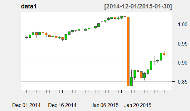
Can you see the big daily candle? This was the day when SNB suddenly announced unpegging CHF from EUR shocking the currency market. First we need to find log returns than we need to find the max and min of the log returns and plot the histogram of log returns.
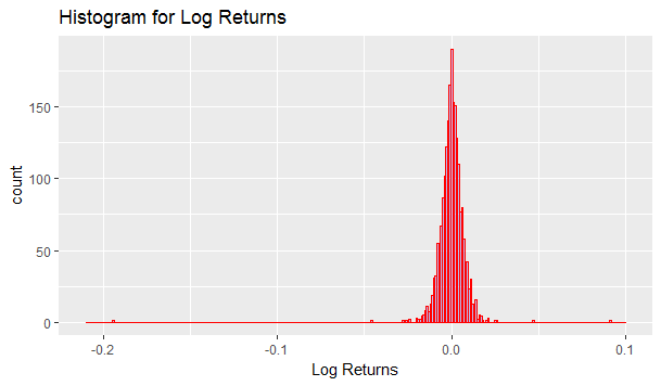
> logReturn <- diff(log(data1$Close))
> logReturn <- logReturn[!is.na(logReturn)]
> summary(logReturn)
     Index                         Close
 Min.   :2009-08-25 00:00:00   Min.   :-1.943e-01
 1st Qu.:2011-08-22 00:00:00   1st Qu.:-3.413e-03
 Median :2013-08-12 00:00:00   Median : 1.105e-05
 Mean   :2013-08-10 14:38:18   Mean   :-4.884e-05
 3rd Qu.:2015-07-30 00:00:00   3rd Qu.: 3.456e-03
 Max.   :2017-07-26 00:00:00   Max.   : 9.093e-02
> library(ggplot2)
> qplot(logReturn,
+       geom="histogram",
+       binwidth = 0.001,
+       main = "Histogram for Log Returns",
+       xlab = "Log Returns",
+       fill=I("blue"),
+       col=I("red"),
+       alpha=I(.2),
+       xlim=c(-0.21,0.1))
Above, you can see the minimum log return which is -0.19. Maximum log return is 0.09. ignore the summary for IndexBelow is the histogram of log returns.
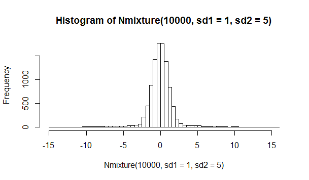
Normal distributions have one major problem. It’s kurtosis is always 3. This means that a normal distribution cannot model events that are rare like the one USDCHF event that happened on 15th Jan 2015. First we need to build a normal mixture model. As said, normal distribution has one major problem. It’s kurtosis is always 3. We can increase the kurtosis to 10, 20 and even 30 by building normal mixture models. Below is the code that builds a sample normal mixture model based on 2 normal distribution.
> Nmixture <- function(N,sd1,sd2=0,thresh=0.9) {
+   variates = vector(length=N)
+   U = runif(N)
+   for(i in 1:N)
+     variates[i] = rnorm(1,0,sd=sd1)
+   if(sd2 != 0) { #only mixture if sd2 != 0
+     for(i in 1:N)
+       if(U[i] >= thresh)
+         #replace original variate with mixture variate
+         variates[i] = rnorm(1,0,sd=sd2)
+   }
+   variates
+ }
> hist(Nmixture(10000,sd1=1,sd2=5),breaks=50)
Below is the plot of simulated normal mixture model.
Important point that we need to determine before we proceed is how many trading days there are in 1 year for a currency market. New York Stock Market is closed for 2 days Saturday and Sunday every week. This means it is closed 8 days in a month and 96 days in a years which gives 365-96=251 days in a year. So NYSE is trading 251 days in a year. What about the currency market? Unlike NYSE, currency market is not a centralized market. Since the currency market is decentralized and opened all the time in different time zones, if we do the calculations we will find that it is closed 1.5 days in a week instead of 2 days. This happens because the Asian Market Session starts on Sunday night in US and the NY Market Session closes on Saturday night so essentially we have the market closed only 1.5 days over the weekend. So we have 285 trading days.Some analyst use 252 trading days others use 365 trading days for currency market.
We will be using a jump model. We will use a binomial random variable with n=281 for modelling the jump that occurred on 15th Jan 2015. Before the jump we will use one normal distribution and after the jump we will use another normal distribution. First we will need to calculate the volatility for the previous year starting from 1st Jan 2014 and 1st Jan 2015.
> data3 <- data1["2014-01-01/2015-01-01"]
> head(data3)
              Open    High     Low   Close Volume
2014-01-02 0.89277 0.90289 0.89232 0.89906  54678
2014-01-03 0.89911 0.90580 0.89894 0.90516  39916
2014-01-06 0.90494 0.90705 0.90202 0.90411  41156
2014-01-07 0.90404 0.90991 0.90357 0.90910  39643
2014-01-08 0.90912 0.91274 0.90769 0.91120  50305
2014-01-09 0.91123 0.91246 0.90633 0.90692  50724
> logReturn <- diff(log(data3[,4]))
> logReturn <- logReturn[!is.na(logReturn)]
> sd1 <- sd(logReturn)
> sd1
[1] 0.004180564
Above we calculated the daily volatility based on past year log returns. Lets calculate the extreme event how many standard deviations away it was from the mean.
> meanUSDCHF <- mean(logReturn)
> x <- data2[(nrow(data2)-11),4]
> (x-meanUSDCHF)/sd1
              Close
2015-01-15 200.5534
You can see on 2015-01-15, USDCHF closing price was a whopping 200 standard deviations away from the mean. This was a very very extreme move that happened in a very short period of time. During this time, market stopped working. Stop losses that had been placed by the traders were not triggers as there was no one to take the other side of the trade. Many traders lost their trading accounts and still had to pay thousands of dollars of losses to their brokers. So it is very important for us to model these extreme events. This extreme events caused havoc with the global markets. But this is not the only extreme event that we are witnessing. As said above GBPUSD also suffered a flash crash. S&P 500 and Dow Jones have also suffered sudden flash crashes so we should be very careful. These extreme events can play havoc with the markets.After the extreme event on 15h Jan, USDCHF stabilized in the next 15 days.
> logReturn <- diff(log(data2[(nrow(data2)-21):nrow(data2),4]))
> logReturn <- logReturn[!is.na(logReturn)]
> sd2 <- sd(logReturn)
> sd2
[1] 0.04498347
> sd2/sd1
[1] 10.76014
You can see above, in Jan 2015, USDCHF volatility was 10 times the normal volatility. If we use a normal distribution, 99% of the data is contained within 3 standard deviations from the mean. In this case we have seen price moves 200 standard deviation from the mean. This is due to the fact the USDCHF has been moving in a tight band before the peg. Once the peg was removed, volatility sky rocketed. We will be using the following three level mixture model for USDCHF extreme event.
- We will use a binomial random variable. Before the USDCHF extreme event it will be 0 and we will use a normal distribution with small standard deviation of sd1 to model the closing price log return series.
- On the extreme event, our binomial random variable becomes 1 and we choose a normal distribution with standard deviation of sd1 which we have shown above to be 200 time sd1.
- After the extreme event we choose a normal distribution with a standard deviation of sd2 which is 10 times sd1 as we have shown it above.
We will use this model for USDCHF. This model is based on the extreme event that took place on 15th Jan 2015.
> library(tseries)

    ‘tseries’ version: 0.10-40

    ‘tseries’ is a package for time series analysis and computational
    finance.

    See ‘library(help="tseries")’ for details.

> tnmixture <- function(N,sd1,sd2=0,sd3=0)
+   #three level mixture with state changes
+ {
+   variates = vector(length=N)
+   mode = 1
+   B = rbinom(365,1,1/365)
+   for(i in 1:N)
+     variates[i] = rnorm(1,0,sd=sd1)
+   if(sd2 != 0) { #only mixture if sd2 != 0
+     for(i in 1:N)
+       if(B[i] == 1) {
+         mode = 2
+         #replace original variate with mixture variate
+         variates[i] = rnorm(1,0,sd=sd2)
+         print(sd2)
+         print(variates[i])
+       } else if (mode == 2) {
+         variates[i] = rnorm(1,0,sd=sd3)
+       }
+   }
+   variates
+ }
First we need the above code that defines a three level mixture model.