Algorithmic trading is the future. Today more than 80% of the trades that are being placed at NYSE are by algorithms. Wall Street firms employ maths and physics PhDs who develop sophisticated algorithmic trading systems that are then unleashed on the markets. Did you read the post on USDCHF extreme monte carlo model? These algorithmic trading systems monitor the market round the clock and buy and sell as programmed. In this post I will discuss Dynamic Time Warping Algorithm (DTW) that has been successfully applied in speech recognition. Can we use DTW in algorithmic trading? This will be the topic of this post. If you are a retail trader then you should know that most of the time you are trading against these algorithms. Either these algorithms lose which is very had and you win or you lose and they win. Chances are you will lose 99% of the time against these algorithms.
Did you notice that traditional technical analysis indicators have become totally useless. Why? You might ask. Answer is simple. These trading algorithms that are based on advanced stochastic calculus concepts have totally made traditional technical analysis useless. Did you read the post on how to code a trailing stop loss? When price moves these algorithms are far ahead of you in determining the market direction and entering in the correct direction. Lose heart? Not at all. Change is the law of life. You should also embrace algorithmic trading and start developing your own systems. As a trader, you should learn MQL4/MQL4 plus one programming language like Python or R. Python is a general purpose modern object oriented language. Learning Python is easy. Just will require a little bit of effort. Let’s now discuss Dynamic Time Wrapping algorithm and how we can use it in trading.
Dynamic Time Warping DTW Algorithm
Dynamic Time Warping (DTW) algorithm is used to measure the optimal alignment between two time series. DTW has been successfully used in speech recognition and many other areas. The objective of DTW algorithm is to compare two time series. Meet John Simmons a mathematician who became a billionaire Hedge Fund Manager. If you have learned technical analysis you should have learned by now that when we look at price charts we are looking for certain patterns that can predict the future. In the past, we have found those price patterns to predict big moves in the market. Well known price patterns that traders use in trading are the head and shoulder pattern, double top and double bottom pattern, wedges, flags and pennants. Traders also use candlestick patterns in predicting the short term price movement. Read this post on trading with double bottom pattern.
Dynamic Time Warping DTW has been successfully used in speech recognition. When we are dealing with currency price data or for that matter the stock market price data, we are dealing with a general class of data known as financial time series data. Financial time series data has some peculiar properties that are not shared by other time series data. The most important peculiarity is the volatility clustering. Now as said above, trading is all about finding patterns in the data that can predict the future. When we are dealing with financial time series data, we are dealing with a fuzzy pattern which is approximate in nature. If you have ever tried to code candlestick patterns, you might have come across this problem of how to code a vague and imprecise pattern which is basically fuzzy in nature. This problem arises because humans are very good at visually identifying these vague and imprecise fuzzy patterns. But when we try to code these patterns, we find it difficult to identify them using computer algorithms. Watch this 50 minute documentary on the Crash of British Pound.
This same problem of matching the exact same words spoken by two or more different persons was successfully solved using the DTW algorithm. For example a person may say a sentence in 30 seconds while another person may say that exact same sentence in more than 60 second even though the words are the same. Same sentences imply that two time series are same but are stretched relative to one another. This is what we do in dynamic time wrapping. We match two time series and try to align them. In Dynamic Time Wrapping, we identify different wrapping pattern between points in the two different time series. For this we need a distance measure which can be the absolute distance also known as Manhattan distance or it can be the square of the difference which is known as the Euclidean distance. There are other more complicated distance measures also like Mahalanobis distance. Once we have the distance measured between the points of the two time series, we try to minimize this total wrapping distance between the two time series.
Dynamic Time Warping algorithm has been applied to many areas now in addition to speech recognition. People have applied DTW algorithm to financial time series analysis as well and reported results that have above 70% accuracy. As said above, we use DTW to compare two time series. DTW allows us to compare two series that can be compressed or expanded relative to each other. We can use DTW to compare a high frequency financial time series with a low frequency financial time series. This is precisely what we will do in this post. Watch this 1 hour video in which a millionaire forex trader explains his trading strategy that uses no stop loss.
In this post we will check if we can adapt DTW algorithm for trading. We will build a few trading models that use DTW algorithm and make predictions and then measure the accuracy of our trading model. Instead of trading live with a rough idea, this is what you should learn to do. If you have a trading strategy, write it down. Once you have written it, try to code it in Python/R and then simulate it on the historical market data. Measure the performance of your trading strategy. If the winrate is above 70%, you above you have a good trading strategy. But this would be your first step. You will have to test the trading strategy on different currency pairs and see how it works overall. If you have good performance something like 70% winrate overall, you can then tweak the trading strategy for each currency pair and check if it improves the performance for that currency pair.
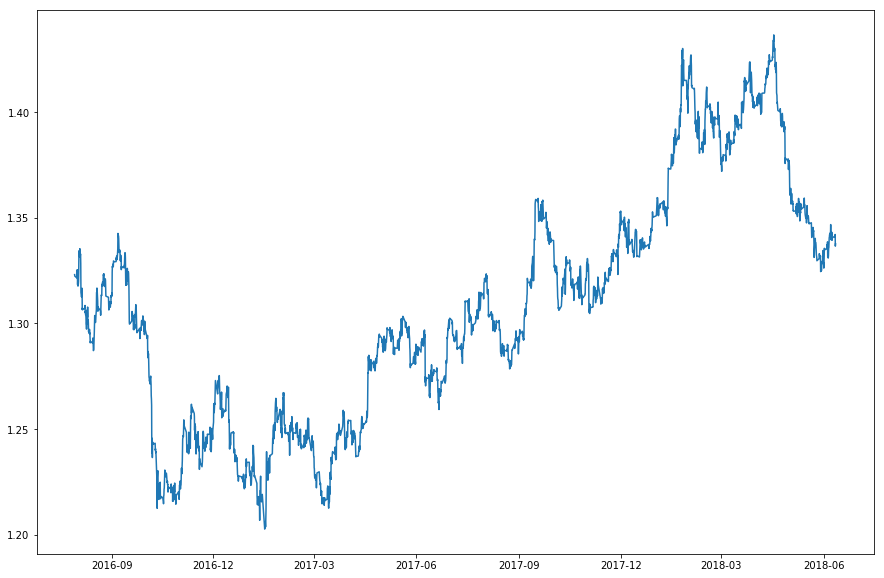
Let’s start with our first DTW trading model first we need to read the data. We will be dealing with intraday data. Let’s read GBPUSD 240 minute data!
import pandas as pd
import numpy as np
#import talib
#from pandas_datareader import data, wb
import matplotlib.pyplot as plt
pd.set_option('display.max_colwidth',200)
#define function to read the data from the csv file
def get_data(currency_pair, timeframe):
    link='D:/Shared/MarketData/{}{}.csv'.format(currency_pair,\
                               timeframe)
    data1 = pd.read_csv(link, header=None)
    data1.columns=['Date', 'Time', 'Open', 'High', 'Low',
                'Close', 'Volume']
    # We need to merge the data and time columns
    # convert that column into datetime object
    data1['Datetime'] = pd.to_datetime(data1['Date'] \
         + ' ' + data1['Time'])
    #rearrange the columnss with Datetime the first
    data1=data1[['Datetime', 'Open', 'High',
                 'Low', 'Close', 'Volume']]
    #set Datetime column as index
    data1 = data1.set_index('Datetime')
    return(data1)

df = get_data('GBPUSD', 240)
df.shape
df.head()
df=df.iloc[-3000:]
This is what I have done. First I defined a function that we can use to import the market data csv file. I can download the market data for any currency pair any timeframe foom MT4. Just use tools>History and you can download the csv file for any currency pair any time frame. Now I need to read that csv file into a dataframe. I use pandas library to read the data using the function that I have defined in the above code. This was the first step.
Testing A Simple Trading Strategy
Let’s test a very simple trading strategy. We are trading on H4 chart. Let’s do a simple thing. We buy at the open of the daily candle and sell at the close of the daily candle. We call this IntraDay Trading Strategy. If price goes up we make a profit and if price goes down we make a loss. We are not using a stop loss at this stage. If at the end of the day, closing price is above the open price we have a winner. On the other hand, if we have closing price below the open, we have a loser. Check this 42-252 SMA Trend Trading Strategy. Important thing when we have a new trading idea is to test it on historical data and check what was its performance on that data. This is no guarantee about the future but testing on the historical data can give a rough idea how things will go in live trading. First we need to develop a performance matrix. I have defined a function that we will give the trading strategy stats. We do that below:
#calculate the trading strategy stats
def getStats(s):
    s=s.dropna()
    wins=len(s[s>0])
    losses=len(s[s<0])
    breakEven=len(s[s==0])
    meanWins=round(s[s>0].mean(),3)
    meanLosses=round(s[s<0].mean(),3)
    winRatio=round(wins/losses,3)
    avgTrade=round(s.mean(),3)
    stdDev=round(np.std(s),3)
    maxLoss=round(s.min(),3)
    maxWin=round(s.max(),3)
    trades=len(s)
    percentageWin=round(wins/trades,3)
    print('Trades:', trades,\
          '\nWins:', wins,\
          '\nLosses:', losses,\
          '\nBreakven:', breakEven,\
          '\nWin/Loss Ratio:', winRatio,\
          '\nMean Win:', meanWins,\
          '\nMean Loss:', meanLosses,\
          '\nMean Trade:', avgTrade,\
          '\nStandard Deviation:', stdDev,\
          '\nMaximum Loss:', maxLoss, \
          '\nMaximum Win:', maxWin,\
          '\nPercentage Winners:', percentageWin
          )
Let's check the performance using H4 GBPUSD data.
df = get_data('GBPUSD', 240)
df.shape
df.head()
df=df.iloc[-3000:]
Now we need to know the daily candle open and the daily candle close for testing this strategy. Using pandas we can easily do that. Pandas is one of the main reasons for the increasing popularity of python as the language of choice for data science, machine learning and deep learning.
If you are a trader, I would suggest you should learn Python. It is an easy language to learn. You can test your trading ideas very easily using Python.
#make a date column
df1=df.copy()
df1['Date'] = [i.date() for i in df1.index]
df1['DailyOpen'] = df1.groupby('Date').Open.transform(\
  lambda s: s[0])
df1['DailyClose'] = df1.groupby('Date').Close.transform(\
  lambda s: s[0])
In the above code, I have made a date column in the dataframe. Now we have two more columns, DailyOpen and DailyClose that give us the open and close of the daily candle. We calculate the intraday returns using these daily open and daily close.
intraDayRtn=100*(df1['DailyClose']-df1['DailyOpen'])/\
df1['DailyOpen']
#remove the duplicate rows
intraDayRtn = intraDayRtn[intraDayRtn.index.hour==00]
There were duplicate rows that I removed using the last command in the above code. Below are the statistics for this very simple trading strategy:
getStats(intraDayRtn)
Trades: 479
Wins: 269
Losses: 210
Breakven: 0
Win/Loss Ratio: 1.281
Mean Win: 0.093
Mean Loss: -0.08
Mean Trade: 0.017
Standard Deviation: 0.119
Maximum Loss: -0.35
Maximum Win: 0.829
Percentage Winners: 0.562
The winrate for this very simple trading strategy is 56%. This is a simple trading strategy that has a winrate of 56%. Keep this in mind, we have no stop loss for this strategy. In the above statistics you can check the maximum loss was 35%. This can be taken as the max drawdown of this trading strategy.We should never trade without a stop loss. This is what we can do. Use the open H4 candle low as the stop loss and again test the trading strategy and see what is the winrate and what is the maximum drawdown. Trading is a long term thing. If you can win more trades in the longterm as compared to losing, you will make a profit. So trading is intricately linked with statistics.
DTW Dynamic Time Warping Algorithm
Let' check if we can use the DTW algorithm and improve the winrate. Below I have developed the python code that a new trading strategy that uses Dynamic Time Wrapping.
##Dynamic Time Wrapping Trading Model
from scipy.spatial.distance import euclidean
from fastdtw import fastdtw
#create function to calculate distance between two time series
def dtwDist(x,y):
    distance, path=fastdtw(x,y, dist=euclidean)
    return distance

tSeries=[]
tlen=6
for k in range(tlen, len(df), tlen):
    pctc=df['Close'].iloc[k-tlen:k].pct_change()[1:].values*100
    res=df['Close'].iloc[k-tlen:k+1].pct_change()[-1]*100
    tSeries.append((pctc,res))
tSeries[0]

distPairs=[]
for k in range(len(tSeries)):
    for j in range(len(tSeries)):
        dist=dtwDist(tSeries[k][0], tSeries[j][0])
        distPairs.append((k,j,dist,tSeries[k][1], \
                          tSeries[j][1]))

distFrame=pd.DataFrame(distPairs, columns=['A', 'B', \                 ##A
        'Distance', 'A Return', 'B Return'])
sf=distFrame[distFrame['Distance'] > 0].sort_values(['A', 'B']).\
   reset_index(drop=1)
sfe=sf[sf['A'] < sf['B']]                                              ##A
winf=sfe[(sfe['Distance'] <=1)&(sfe['A Return']>0)]
plt.plot(np.arange(5),tSeries[6][0])
plt.plot(np.arange(5), tSeries[len(tSeries)-1][0])
#evaluate the DTW trading strategy
excluded={}
returnList=[]
def getReturns(r):
    if excluded.get(r['A']) is None:
        returnList.append(r['B Ret'])
        if r['B Ret'] < 0:
            excluded.update({r['A']:1})

winf.apply(getReturns, axis=1)
getStats(pd.Series(returnList))
Let's check the stats for this new trading strategy!
Trades: 465
Wins: 222
Losses: 242
Breakven: 1
Win/Loss Ratio: 0.917
Mean Win: 0.124
Mean Loss: -0.157
Mean Trade: -0.022
Standard Deviation: 0.203
Maximum Loss: -0.959
Maximum Win: 0.882
Percentage Winners: 0.477
The new trading strategy has infact a poorer winate as compared to our benchmark simple trading strategy. Max drawdown is also worse. What are we doing? This is a illustration of what happens when you try to use machine learning without putting much thought into it.
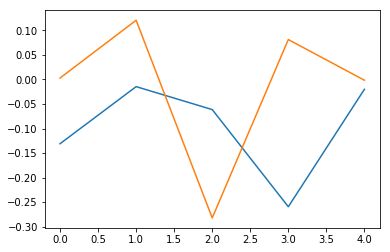
In the above screenshot you can see that the DTW algorithm is not correctly aligning the two time series. This we need to correct if we want to improve our DTW Trading Strategy. Did you check Quantopian. One problem with dynamic time wrapping algorithm is that it takes some time to give results. So we may not be able to use it on high frequency timeframes like 1 minute or 5 minutes but we can use it on 240 minutes and 60 minutes timeframe. Now let's start building a new DTW Trading Strategy that can give good results. In the above DTW Trading Strategy we used H4 candles. Instead of looking at the returns let's check by working directly with the closing price and see what did fastDTW produced.
10**4*(df['Close'][-1]-df['Close'][0])
Out[74]: 145.50000000000063

10**4*(df['Close'][max(sfe['B'])]-df['Close'][min(sfe['A'])])
Out[75]: -301.00000000000017

df.iloc[min(sfe['A'])]
Out[76]:
Open         1.32675
High         1.32706
Low          1.32222
Close        1.32309
Volume    7644.00000
Name: 2016-07-29 16:00:00, dtype: float64
#plot the closing price
plt.plot(np.arange(min(sfe['A']),max(sfe['B'])),\
         df['Close'][min(sfe['A']):max(sfe['B'])])
10**4*(df['Close'][max(sfe['B'])]-df['Close'][21])
Out[88]: -398.6000000000023
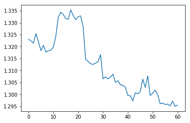
You can see the H4 closing price total movement was only 145 pips while the fastDTW algorithm was able to catch the closing price down move that made 301 pips. But if you look at the above screenshot, you will see that if we had entered at min(sfe['A']), our stop loss would have been only 40 Pips (High - Close) and the stop loss would have been hit as price went up before price started to move down. Closing price at index 21 gives us the best results by catching a big move of almost 400 pips and stop loss of 18 pips.
What we need to do is work more and find an entry point with risk that is less than 15 pips. This means moving towards a lower timeframe like M30. I once again read the M30 data and start the fastDTW algorithm. It takes time like 2-3 minutes to do the calculations. DTW algorithm is of order O(mn) where m is the length of first time series and n is the length of second time series. Right now we are not concerned with this time as we want to see whether fastDTW can be used in building a trading strategy or not.
It is always a good idea to get familiar with the algorithm before you can use it. What I have done is Let's check what fastDTW algorithm has produced so far. If you check distFrame has got more than 10,000 rows. We have converted the list distPairs into a pandas dataframe distFrame and named the columns as A, B, Distance, A Return and B Return (check code marked ##A). After that we removed the distance 0 and resorted the distFrame in an ascending values and reset the index as a number of rows that had distance zero were removed. Distance zero only means same points in the time series so we value in keeping that. After that we removed all those rows that had B lower than A which meant time series points that were in future coming before time series points that were before them in the past. So we removed them. Let's add one more condition and check if we have some information that we can utilize in our trading strategy.
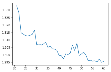
sfe[(sfe['A'] == min(sfe['A']))&(sfe['B'] == max(sfe['B']))]
10**4*(df['Close'][max(sfe['B'])]-df['Close'][min(sfe['A'])])
Out[51]: 249.29999999999896

##plot the price movement
plt.plot(np.arange(103),df['Close'][0:103])

10**4*(df['Close'][-1]-df['Close'][0])
Out[54]: 296.60000000000019

df.iloc[min(sfe['A'])]
Out[56]:
Open         1.29253
High         1.29324
Low          1.29191
Close        1.29280
Volume    1334.00000
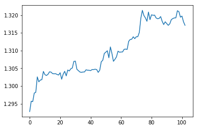
This condition tells us the row which has A minimum and B maximum. Let's check whether there is some information in it. You can see if we take the last closing price and subtract it from the first in our original closing price data, we find that in total of 5000 M30 candles, total price movement was only 296 pips. In the above code, you can see fastDTW was able to detect the best entry M30 candle and the best exit M30 candle and gave us a price movement of 249 pips. The stop loss was only 10 pips. If you have been reading my blog, I always look for entries with the smallest possible risk. We haven't made any forecast with fastDTW. Forecasting or predicting the price in the future is what is required when building a trading strategy. We have only analyzed the historical closing price data. So let's see if we can make predictions using fastDTW.
If you are reading my post intently than you must have seen the though process in developing a trading strategy. Our aim is to catch the big moves with as small a stop loss as possible and achieve a winrate something that is above 80%. This is the main aim. What we are doing is checking whether the dynamic time warping algorithm can help us in building a forex trading strategy that has an average stop loss of 15 pips and an average take profit of 200 pips. Keeping on reading this post on how to use DTW Dynamic Time Warping in trading as I am going to update this blog post with new results after a few days as I have said, we haven't done any forecasting yet, we are just exploring the dynamic time warping algorithm and checking how can we use it in building a good trading strategy.